Chapter 1: Introduction to Simulated Annealing #

Section 1: What is Simulated Annealing? #

1.1 Overview #

Simulated annealing (SA) is a powerful probabilistic optimization technique used to approximate the global optimum of a given function. As a software developer or engineer, you may encounter complex optimization problems in various fields, such as engineering, economics, or computer science. Simulated annealing provides a robust and efficient approach to tackle these challenges.

The algorithm draws inspiration from the physical process of annealing in metallurgy, where a material is heated and then slowly cooled to reduce defects and minimize energy states. In the context of optimization, simulated annealing uses a temperature parameter to control the search process, allowing it to escape local minima by accepting worse solutions with a certain probability. This unique feature enables the algorithm to explore a large search space effectively and find near-optimal solutions, even in the presence of numerous local minima.

Simulated annealing offers several advantages over other optimization techniques. Its ability to handle large search spaces and its robustness to initial conditions make it a valuable tool in solving real-world problems. By the end of this chapter, you will have a solid understanding of the fundamental concepts behind simulated annealing and be ready to implement it in your own projects.

1.2 Historical Background #

The origins of simulated annealing can be traced back to the Metropolis algorithm, developed by Metropolis, Rosenbluth, and Teller in 1953. The Metropolis algorithm was initially used to simulate the evolution of a solid to thermal equilibrium, employing a probabilistic approach to determine the acceptance of state transitions.

In 1983, Kirkpatrick, Gelatt, and Vecchi made a groundbreaking contribution by adapting the Metropolis algorithm to optimization problems. They introduced the concept of temperature and annealing schedule, which allowed the algorithm to escape local minima and converge towards the global optimum. Their seminal paper laid the foundation for the development and application of simulated annealing in various domains.

Independently, Černý discovered the algorithm in 1985, further validating its potential as an optimization technique. In 1988, Hajek provided a convergence proof for simulated annealing, establishing its theoretical foundations. Ingber’s introduction of adaptive simulated annealing in 1989 further enhanced the algorithm’s performance and adaptability.

As simulated annealing gained popularity, it found applications in diverse fields such as operations research, physics, and materials science. Researchers and practitioners developed various variants and extensions, including parallel simulated annealing and quantum annealing, to tackle specific problem domains and improve efficiency.

Simulated annealing has been compared and contrasted with other optimization techniques, such as genetic algorithms and particle swarm optimization. While each method has its strengths and weaknesses, simulated annealing remains a powerful and widely-used approach, particularly for problems with large search spaces and complex energy landscapes.

Section 2: Physical Inspiration of the Algorithm #

2.1 Metallurgical Annealing Process #

To understand the inspiration behind simulated annealing, let’s dive into the physical process of annealing in metallurgy. Annealing involves heating a metal to a high temperature, allowing its atoms to move freely within the structure. As the metal is slowly cooled, the atoms gradually settle into a low-energy crystalline configuration. This controlled heating and cooling process offers several benefits:

• Reduces defects and dislocations in the material
• Enhances strength, ductility, and other desirable physical properties

The effectiveness of the annealing process depends on several key factors:

1. Initial temperature: The metal must be heated to a sufficiently high temperature to overcome energy barriers and enable atomic movement.
2. Cooling rate: The rate at which the metal is cooled determines the final crystalline structure. Slower cooling allows atoms more time to find the lowest energy configuration.
3. Material properties: The specific heat capacity, thermal conductivity, and other properties of the metal influence the annealing process.

By carefully controlling these factors, metallurgists can optimize the annealing process to achieve the desired material properties.

2.2 Analogy to Optimization #

The physical process of annealing serves as a powerful analogy for optimization in simulated annealing. Just as heating and slow cooling enable atoms to settle into low-energy states in metallurgy, the simulated annealing algorithm explores the search space and gradually converges towards optimal solutions.

In simulated annealing, the “temperature” parameter plays a crucial role in controlling the search process. At high temperatures, the algorithm is more likely to accept worse solutions, allowing it to explore a wide range of possibilities and escape local minima. As the temperature decreases, the algorithm becomes more selective, focusing on promising regions of the search space.

This annealing-inspired optimization process can be summarized as follows:

1. Initialize with a high “temperature” to allow exploration of the search space
2. Gradually lower the “temperature” to focus on promising regions
3. Accept worse solutions probabilistically to escape local minima

The key aspects of the analogy include:

• Temperature control: Balancing exploration and exploitation
• Slow cooling: Systematic convergence towards optimal solutions
• Energy minimization: Optimization of the objective function

While the analogy between physical annealing and simulated annealing is compelling, it’s important to note some differences:

• Discrete vs continuous state space: Physical annealing deals with discrete atomic configurations, while optimization often involves continuous variables.
• Stochastic vs deterministic transitions: Simulated annealing relies on probabilistic acceptance of new solutions, while physical annealing follows deterministic laws of physics.
• Metallurgical properties vs optimization objectives: The goals of physical annealing relate to material properties, while simulated annealing aims to optimize a specific objective function.

Despite these differences, the physical inspiration behind simulated annealing provides a powerful framework for tackling complex optimization problems.

Section 3: Basic Concepts in Continuous Function Optimization #

3.1 Understanding Optimization Landscapes #

An optimization landscape is a powerful tool for visualizing the solutions to an optimization problem. Imagine a topographical map, where the decision variables (such as x and y) represent the coordinates on the map, and the objective function value (z) represents the elevation. The optimization landscape is a visual representation of this concept, allowing us to see the “hills,” “valleys,” and “plateaus” that correspond to different solutions.

In a two-dimensional optimization landscape, we can picture the objective function as a curve, with peaks representing high values and troughs representing low values. In three dimensions, the landscape becomes a surface, with contours indicating areas of equal objective function value.

The goal of optimization is to navigate this landscape and find the lowest point (for minimization problems) or the highest point (for maximization problems). By visualizing the optimization landscape, we can better understand the challenges and opportunities in finding the optimal solution.

3.2 Local Minima and Global Minima #

When exploring an optimization landscape, it’s crucial to understand the difference between local minima and global minima. A local minimum is a solution that is better than all nearby solutions but not necessarily the best solution overall. In contrast, the global minimum is the best solution in the entire search space.

To illustrate this concept, imagine a hiker trying to find the lowest point in a mountain range. A local minimum would be a valley that is lower than all the surrounding peaks, but there might be an even lower valley elsewhere in the range. The global minimum, on the other hand, would be the absolute lowest point in the entire mountain range.

Traditional optimization methods often struggle with local minima, as they can get stuck in these suboptimal solutions and fail to explore other parts of the search space. This is where simulated annealing shines. By allowing the acceptance of worse solutions with a certain probability, simulated annealing can escape local minima and explore more of the optimization landscape, increasing the chances of finding the global minimum.

3.3 Importance of Initial Conditions #

The starting point of an optimization algorithm can have a significant impact on its path and the final outcome. In the context of an optimization landscape, the initial conditions determine where the algorithm begins its journey.

If the initial starting point is near the global minimum, the algorithm may converge quickly to the optimal solution. However, if the starting point is close to a local minimum, the algorithm may struggle to escape that suboptimal region and find the global minimum.

Strategies for choosing initial conditions include random initialization, where the starting point is chosen randomly within the search space, and domain knowledge-informed initialization, where prior knowledge about the problem is used to select a promising starting point.

In simulated annealing, the choice of initial conditions can influence the algorithm’s performance. Better initial conditions can lead to faster convergence and higher-quality solutions. However, the probabilistic nature of simulated annealing allows it to overcome poor initial conditions more effectively than many other optimization algorithms.

Section 4: Pseudocode of Simulated Annealing #

4.1 High-Level Overview #

Pseudocode is a valuable tool for understanding the structure and logic of an algorithm without getting bogged down in language-specific syntax. It provides a clear, concise representation of the key steps involved in a process. Let’s take a look at the high-level pseudocode for the simulated annealing algorithm:

1. Initialize solution and temperature
2. While not converged:
   2.1 Generate new solution
   2.2 Calculate change in objective function
   2.3 If improvement or acceptance probability met:
       2.3.1 Accept new solution
   2.4 Reduce temperature
3. Return best solution found

This pseudocode highlights the core components of simulated annealing: initialization, solution generation, acceptance criteria, and temperature reduction. By understanding these key steps, you’ll be well on your way to implementing a simulated annealing algorithm in your optimization projects.

4.2 Explanation of Each Step #

Let’s dive deeper into each step of the simulated annealing pseudocode to gain a better understanding of how the algorithm works.

4.2.1 Initialization #

The first step in simulated annealing is to initialize a valid starting solution and set an appropriate initial temperature. The initial solution can be generated randomly or using domain-specific knowledge to provide a good starting point for the optimization process.

Choosing the right initial temperature is crucial. It should be high enough to allow the algorithm to explore a wide range of solutions but not so high that it takes too long to converge. Common techniques for setting the initial temperature include using a fixed value based on problem characteristics or experimentally determining a suitable temperature range.

4.2.2 Solution Generation #

In each iteration of the simulated annealing algorithm, a new solution is generated by modifying the current solution. This is done by defining a neighborhood structure, which determines what constitutes a “neighbor” solution. Common techniques for generating neighbors include:

• Perturbation: Randomly modifying one or more components of the current solution
• Swaps: Exchanging the values of two or more components in the solution

The size of the neighborhood can be adjusted to balance exploration and exploitation. Larger neighborhoods allow for more extensive exploration of the search space, while smaller neighborhoods focus on fine-tuning existing solutions.

4.2.3 Acceptance Criteria #

Once a new solution is generated, the simulated annealing algorithm must decide whether to accept it as the current solution. The Metropolis criterion is used for this purpose:

• If the new solution improves the objective function, it is always accepted.
• If the new solution worsens the objective function, it is accepted with a probability based on the current temperature and the magnitude of the objective function change.

The acceptance probability is calculated using the following formula:

P(accept) = e^(-ΔE / T)

where e is the exponential function, ΔE is the change in the objective function value, and T is the current temperature.

Occasionally accepting worse solutions allows the algorithm to escape local minima and explore more of the search space, increasing the chances of finding the global optimum.

4.2.4 Temperature Reduction #

As the simulated annealing algorithm progresses, the temperature is gradually reduced according to a cooling schedule. Common cooling schedules include linear and exponential decay. The choice of cooling schedule involves a trade-off between solution quality and runtime. Slower cooling generally leads to better solutions but longer runtimes, while faster cooling may converge more quickly but risks getting stuck in suboptimal solutions. We’ll explore cooling schedules in more detail in the next chapter.

Section 5: Choosing a Test Problem #

5.1 Introduction to a Multi-Modal Test Function #

To demonstrate the power and versatility of simulated annealing, we’ll be using a multi-modal function as our test problem. The function we’ve chosen is:

f(x) = sin(x) + sin(10 * x / 3)

This function is particularly well-suited for showcasing simulated annealing’s ability to escape local minima and find the global minimum in a complex optimization landscape.

Let’s take a look at the graph of this function with input values between -5 and 5:

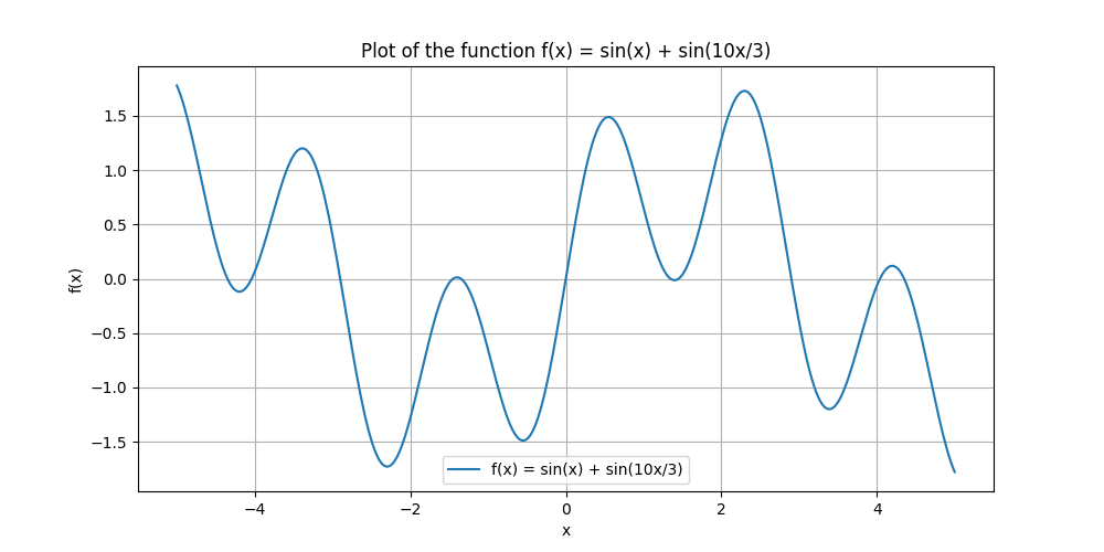
As you can see, the function has multiple local minima (the valleys) and one global minimum (the deepest valley). This is a classic example of a multi-modal optimization problem, where the challenge lies in finding the global minimum among many local minima.

The global minima (lowest output value) is an input value x ≈ −2.30 with an output value of f(x) ≈ −1.73.

Exercises #

In this exercise, you will implement and visualize the initial stage of the simulated annealing process using the multi-modal test function introduced in the chapter. By generating random sample points and plotting them alongside the target function, you will gain a visual understanding of how simulated annealing begins exploring the optimization landscape.

Exercise 1: Generating Sample Points #

Create a Python function called generate_sample_points that randomly generates a set of initial points within a specified range for the function f(x) = sin(x) + sin(10 * x / 3). Follow these steps:

1. Define the function generate_sample_points that takes the following parameters:

   • num_points: The number of sample points to generate.
   • x_min: The minimum value of the range for generating points.
   • x_max: The maximum value of the range for generating points.

2. Inside the function, use numpy.random.uniform to generate num_points random values between x_min and x_max.

3. Return the generated sample points as a NumPy array.

Exercise 2: Plotting the Target Function #

Plot the multi-modal test function f(x) = sin(x) + sin(10 * x / 3) over the range [-5, 5] using the matplotlib library. Follow these steps:

1. Create a new Python script.

2. Import the necessary libraries: numpy and matplotlib.pyplot.

3. Define the test_function() that takes an numerical argument and returns the computed function value.

4. Generate a set of evenly spaced points within the range [-5, 5] using numpy.linspace.

5. Evaluate the test function for each point using the test_function defined earlier.

6. Create a plot using matplotlib.pyplot.plot to visualize the test function.

7. Add labels, a title, and any other desired formatting to the plot.

Exercise 3: Plotting Generated Points #

Overlay the randomly generated sample points from Exercise 1 on the plot of the target function created in Exercise 2. This will help visualize where the simulated annealing process starts exploring. Follow these steps:

1. Update the script from Exercise 2, call the generate_sample_points function from Exercise 1 to create a set of random sample points.

2. Plot the generated sample points on the same figure as the target function using matplotlib.pyplot.scatter.

3. Adjust the plot labels, title, and formatting as needed to incorporate the sample points.

By completing this exercise, you will have implemented the initial stage of the simulated annealing process and visualized the randomly generated sample points on the optimization landscape. This visualization provides a clear understanding of where the simulated annealing algorithm begins its exploration in search of the global minimum.

Take a moment to observe the distribution of the sample points and consider how they might influence the algorithm’s initial exploration. Experiment with different numbers of sample points and observe how the visualization changes.

Answers #

import numpy as np

def generate_sample_points(num_points, x_min, x_max):
    # Generate num_points random values between x_min and x_max
    sample_points = np.random.uniform(x_min, x_max, num_points)
    return sample_points

import numpy as np
import matplotlib.pyplot as plt

def test_function(x):
    return np.sin(x) + np.sin(10 * x / 3)

# Generate a set of evenly spaced points within the range [-5, 5]
x_values = np.linspace(-5, 5, 400)
y_values = test_function(x_values)

# Create a plot to visualize the test function
plt.plot(x_values, y_values, label='f(x) = sin(x) + sin(10*x/3)')
plt.title('Plot of the Multi-modal Test Function')
plt.xlabel('x')
plt.ylabel('f(x)')
plt.legend()
plt.show()

import numpy as np
import matplotlib.pyplot as plt

def generate_sample_points(num_points, x_min, x_max):
    # Generate num_points random values between x_min and x_max
    sample_points = np.random.uniform(x_min, x_max, num_points)
    return sample_points

def test_function(x):
    return np.sin(x) + np.sin(10 * x / 3)

# Generate a set of evenly spaced points within the range [-5, 5]
x_values = np.linspace(-5, 5, 400)
y_values = test_function(x_values)

# Generate random sample points within the range [-5, 5]
num_points = 50  # Number of sample points
sample_points = generate_sample_points(num_points, -5, 5)
sample_values = test_function(sample_points)

# Plot the target function
plt.plot(x_values, y_values, label='f(x) = sin(x) + sin(10*x/3)')
# Add the randomly generated sample points
plt.scatter(sample_points, sample_values, color='red', label='Sample Points')
plt.title('Initial Sampling in Simulated Annealing')
plt.xlabel('x')
plt.ylabel('f(x)')
plt.legend()
plt.show()

Summary #

Chapter 1 introduced Simulated Annealing (SA), a powerful probabilistic optimization technique inspired by the physical process of annealing in metallurgy. The chapter explored the origins and historical background of SA, drawing parallels between the controlled heating and cooling of materials and the optimization process. Core concepts in continuous function optimization, such as optimization landscapes, local minima, and global minima, were explained in detail. The high-level pseudocode of SA was presented, breaking down each step of the algorithm. Finally, a multi-modal test function was chosen to demonstrate SA’s ability to escape local minima and find the global optimum in a complex optimization landscape.

Key Takeaways #

1. Simulated Annealing is inspired by the physical process of annealing, leveraging controlled temperature changes to navigate complex optimization landscapes and find near-optimal solutions.
2. The algorithm balances exploration and exploitation through a temperature parameter, accepting worse solutions probabilistically to escape local minima.
3. Understanding optimization landscapes, local minima, and global minima is crucial for grasping the challenges and opportunities in finding optimal solutions.

Exercise Encouragement #

Dive into the world of Simulated Annealing by implementing the initial stage of the algorithm and visualizing the randomly generated sample points on the optimization landscape. This hands-on exercise will solidify your understanding of the core concepts and provide a clear picture of how SA begins exploring the search space. Don’t be intimidated by the multi-modal test function - take it step by step, and you’ll gain valuable insights into the inner workings of SA. Your efforts here will lay the foundation for mastering this powerful optimization technique and applying it to real-world problems!

Glossary: #

• Simulated Annealing (SA): A probabilistic optimization technique inspired by the physical process of annealing in metallurgy.
• Annealing: The process of heating a material and then slowly cooling it to reduce defects and minimize energy states.
• Optimization Landscape: A visual representation of the solutions to an optimization problem, with decision variables as coordinates and the objective function value as elevation.
• Local Minimum: A solution that is better than all nearby solutions but not necessarily the best solution overall.
• Global Minimum: The best solution in the entire search space.
• Temperature: A parameter in SA that controls the probability of accepting worse solutions, allowing the algorithm to escape local minima.
• Cooling Schedule: The rate at which the temperature is reduced during the SA process, balancing solution quality and runtime.
• Metropolis Criterion: The acceptance rule in SA, determining whether to accept a new solution based on the current temperature and the change in the objective function value.
• Multi-Modal Function: A function with multiple local minima and one or more global minima, presenting a challenging optimization landscape.
• Numerical Methods: Techniques for finding approximate solutions to mathematical problems, often used when analytical solutions are difficult or impossible to obtain.

Next Chapter: #

In Chapter 2, we’ll explore the role of temperature in Simulated Annealing and examine different cooling schedules, understanding how they affect the search process and the algorithm’s performance in finding optimal solutions.