Chapter 1: Introduction to Particle Swarm Optimization #

1.1 History and Conceptual Foundation #

1.1.1 Origins of PSO #

Particle Swarm Optimization (PSO) was first introduced in 1995 by James Kennedy and Russell Eberhart as a novel optimization algorithm inspired by the social behavior of birds and fish. The goal was to develop a simple yet efficient method for solving complex optimization problems by leveraging the power of collective intelligence.

Kennedy and Eberhart were fascinated by the way birds in a flock and fish in a school could coordinate their movements without any central control. They recognized that these natural phenomena could serve as a metaphor for a new optimization paradigm, leading to the birth of PSO.

1.1.2 Natural Phenomena and Inspiration #

Flocking Behavior in Birds #

Have you ever marveled at the mesmerizing sight of a flock of birds swooping and soaring in unison? This remarkable display of coordination arises from simple local interactions among individual birds. Each bird in the flock adjusts its position and velocity based on the movements of its nearby neighbors, resulting in a collective behavior that appears almost choreographed.

In the context of PSO, each bird in the flock can be thought of as a particle in the swarm. These particles communicate with each other, sharing information about their current positions and velocities. By learning from their neighbors’ experiences, particles can adapt their own movements and collaboratively explore the search space.

Schooling Behavior in Fish #

Similar to birds, fish in a school exhibit a stunning display of collective intelligence. When faced with predators or navigating through complex environments, fish rely on the power of numbers and coordination to enhance their chances of survival.

Each fish in the school maintains a certain distance from its neighbors while aligning its velocity with the group. This allows the school to move as a cohesive unit, responding swiftly to changes in their surroundings. The emergent behavior of the school is a result of simple rules followed by individual fish, showcasing the efficiency and robustness of decentralized decision-making.

Translating Natural Behaviors into Algorithmic Structure #

The PSO algorithm abstracts these natural behaviors into a computational framework. Each particle in the swarm represents a potential solution to the optimization problem at hand. These particles are simple agents with limited individual capabilities, but when they interact and share information, they can collectively solve complex problems.

The movement of particles in PSO is governed by a set of mathematical equations that capture the essence of flocking and schooling behaviors. Particles are attracted towards the best solutions discovered by themselves (personal best) and the swarm as a whole (global best). By striking a balance between individual exploration and social exploitation, the swarm progressively refines its search, converging towards optimal solutions.

The beauty of PSO lies in its simplicity and effectiveness. By drawing inspiration from the collective intelligence observed in nature, PSO provides a powerful tool for tackling optimization challenges across various domains, from engineering and computer science to finance and beyond.

1.2 Core Components of PSO #

1.2.1 Overview of Key Elements #

At the heart of Particle Swarm Optimization (PSO) lie its fundamental building blocks: particles, population, positions, velocities, and the objective function. These core components work together to enable the swarm to explore the search space effectively and converge towards optimal solutions. Let’s dive into each of these elements in more detail.

1.2.2 Particles and Population #

In the context of PSO, particles are the basic entities that navigate the search space. Each particle represents a potential solution to the optimization problem at hand. You can think of particles as agents or individuals within the swarm, each contributing to the collective intelligence of the group.

Particles possess two key attributes: position and velocity. The position of a particle refers to its current location in the search space. It encodes the values of the problem variables that define a specific solution. As the particle moves through the search space, its position is updated based on its velocity.

The velocity, on the other hand, determines the speed and direction of a particle’s movement. It is influenced by various factors, including the particle’s own experience (personal best) and the experience of the swarm as a whole (global best). We’ll explore these concepts in greater detail in the upcoming chapters.

In PSO, particles are organized into a population. The population is essentially a collection of particles that interact and share information with each other. The diversity within the population is crucial for maintaining a balance between exploration and exploitation. By having particles with different positions and velocities, the swarm can effectively explore various regions of the search space while also refining promising solutions.

1.2.3 Position and Velocity #

The position of a particle is more than just a point in the search space; it represents a potential solution to the optimization problem. The position encodes the values of the problem variables, mapping them from the search space to the solution space. For example, if we’re optimizing the weights of a neural network, each particle’s position would represent a specific configuration of those weights.

To evaluate the quality of a particle’s position, we use an objective function. The objective function measures how well a particular solution performs with respect to the optimization goal. It assigns a fitness value to each position, allowing us to compare and rank different solutions. The objective function acts as a guide, steering the particles towards regions of the search space that are more promising.

The velocity of a particle plays a crucial role in its movement through the search space. It determines both the direction and the magnitude of the particle’s motion. The velocity is influenced by several factors, including the particle’s own experience (personal best) and the experience of the swarm (global best). These factors contribute to the particle’s decision on how to adjust its velocity in each iteration.

The interplay between position and velocity is what drives the optimization process in PSO. As particles update their velocities based on personal and social influences, they move to new positions in the search space. These new positions are then evaluated using the objective function, and the fitness values are compared to the particle’s personal best and the swarm’s global best. This feedback loop allows particles to learn from their own experiences and the experiences of others, guiding them towards optimal solutions.

1.3 Basic Mathematical Model #

At the core of Particle Swarm Optimization (PSO) lies a set of mathematical equations that govern the movement of particles through the search space. These equations determine how particles update their positions and velocities based on their own experiences and the experiences of the swarm as a whole. Let’s dive into these equations and explore the parameters that influence particle movement.

1.3.1 Particle Movement Equations #

The movement of particles in PSO is guided by two fundamental equations: the position update equation and the velocity update equation. The position update equation is given by:

x(t+1) = x(t) + v(t+1)

where x(t) represents the current position of the particle, v(t+1) is the updated velocity, and x(t+1) is the new position of the particle. This equation simply states that the new position of a particle is calculated by adding its updated velocity to its current position.

The velocity update equation, on the other hand, is a bit more complex:

v(t+1) = w * v(t) + c1 * r1 * (pbest - x(t)) + c2 * r2 * (gbest - x(t))

Here, v(t) is the current velocity of the particle, w is the inertia weight, c1 and c2 are acceleration coefficients, r1 and r2 are random numbers between 0 and 1, pbest is the particle’s personal best position, and gbest is the global best position found by the entire swarm.

The velocity update equation consists of three main components:

1. The inertia component (w * v(t)): This term represents the particle’s tendency to continue moving in its previous direction.
2. The cognitive component (c1 * r1 * (pbest - x(t))): This term pulls the particle towards its personal best position.
3. The social component (c2 * r2 * (gbest - x(t))): This term attracts the particle towards the global best position found by the swarm.

By combining these components, the velocity update equation balances the particle’s individual experience (cognitive component) with the collective experience of the swarm (social component), while also considering the particle’s previous velocity (inertia component).

Let’s consider a simple example to illustrate the application of these equations. Suppose a particle’s current position is x(t) = (2, 3), its current velocity is v(t) = (1, 1), its personal best position is pbest = (4, 5), and the global best position is gbest = (6, 7). If we set w = 0.8, c1 = 1.5, c2 = 2, and r1 = 0.6, r2 = 0.4, then the updated velocity would be:

v(t+1) = 0.8 * (1, 1) + 1.5 * 0.6 * ((4, 5) - (2, 3)) + 2 * 0.4 * ((6, 7) - (2, 3))
       = (0.8, 0.8) + (1.8, 1.8) + (3.2, 3.2)
       = (5.8, 5.8)

And the new position would be:

x(t+1) = (2, 3) + (5.8, 5.8) = (7.8, 8.8)

1.3.2 Parameters Influencing Movement #

The behavior and convergence of PSO are greatly influenced by the parameters in the velocity update equation. Let’s take a closer look at these parameters and their roles:

1. Inertia weight (w): The inertia weight controls the particle’s tendency to continue moving in its previous direction. A higher inertia weight encourages exploration, allowing particles to venture into new regions of the search space. Conversely, a lower inertia weight promotes exploitation, focusing the search around promising areas. Strategies for setting the inertia weight include using a fixed value, linearly decreasing it over time, or adapting it based on the swarm’s performance.

2. Acceleration coefficients (c1 and c2):

   • The cognitive acceleration coefficient (c1) determines the particle’s inclination to move towards its personal best position. A higher c1 value emphasizes the particle’s individual experience and encourages it to explore the vicinity of its personal best.
   • The social acceleration coefficient (c2) governs the particle’s tendency to move towards the global best position. A higher c2 value prioritizes the collective experience of the swarm and attracts particles towards the best solution found by the entire group.

The values assigned to these coefficients affect the balance between exploration and exploitation. Typically, c1 and c2 are set to values between 1 and 2, with their sum often equal to 4. However, the optimal values may vary depending on the problem and desired convergence behavior.

The interplay between the inertia weight and acceleration coefficients determines the overall convergence behavior of PSO. High inertia weight combined with low acceleration coefficients promotes exploration, allowing particles to broadly search the solution space. On the other hand, low inertia weight and high acceleration coefficients favor exploitation, intensifying the search around promising regions.

By understanding and tuning these parameters, you can fine-tune the performance of PSO for specific optimization problems. Experimenting with different parameter settings and observing their impact on convergence can help you strike the right balance between exploration and exploitation, ultimately leading to more effective optimization results.

1.4 Continuous Function Optimization #

In the realm of optimization, continuous function optimization plays a crucial role in solving real-world problems. Many applications, ranging from engineering design to machine learning, involve finding the best solution within a continuous search space. Particle Swarm Optimization (PSO), originally designed for discrete optimization, can be easily adapted to tackle continuous optimization tasks. In this section, we’ll explore how PSO can be applied to optimize continuous functions, using the Rosenbrock function as a benchmark example.

1.4.1 Introduction to Continuous Optimization #

Continuous function optimization involves finding the minimum or maximum value of a function where the input variables can take on any value within a specified range. In contrast to discrete optimization, where variables are restricted to a set of distinct values, continuous optimization allows for a more fine-grained search over a continuous domain.

PSO can be seamlessly adapted to solve continuous optimization problems by representing particles’ positions as real-valued vectors in the continuous search space. The particles explore the search space, updating their positions and velocities based on their own best-known solution and the swarm’s global best solution, ultimately converging towards the optimal point.

1.4.2 Benchmark Function: The Rosenbrock Function #

To demonstrate the application of PSO in continuous optimization, we’ll use the Rosenbrock function as a benchmark. The Rosenbrock function, also known as the banana function due to its shape, is a commonly used test function for optimization algorithms. It is defined as:

f(x, y) = (1 - x)^2 + 100(y - x^2)^2

The Rosenbrock function is characterized by a global minimum located at (1, 1), where the function value is 0. However, the function has a narrow, parabolic-shaped valley that poses challenges for optimization algorithms to converge to the global minimum.

1.4.2.1 Visualizing the Rosenbrock Function #

To gain a better understanding of the Rosenbrock function’s landscape, let’s visualize it using a contour plot in Python:

import numpy as np
import matplotlib.pyplot as plt

def rosenbrock(x, y):
    return (1 - x)**2 + 100 * (y - x**2)**2

x = np.arange(-2, 2, 0.01)
y = np.arange(-1, 3, 0.01)
X, Y = np.meshgrid(x, y)
Z = rosenbrock(X, Y)

plt.contour(X, Y, Z, 50, cmap='jet')
plt.xlabel('x')
plt.ylabel('y')
plt.title('Rosenbrock Function Contour Plot')
plt.show()

The output looks as follows:

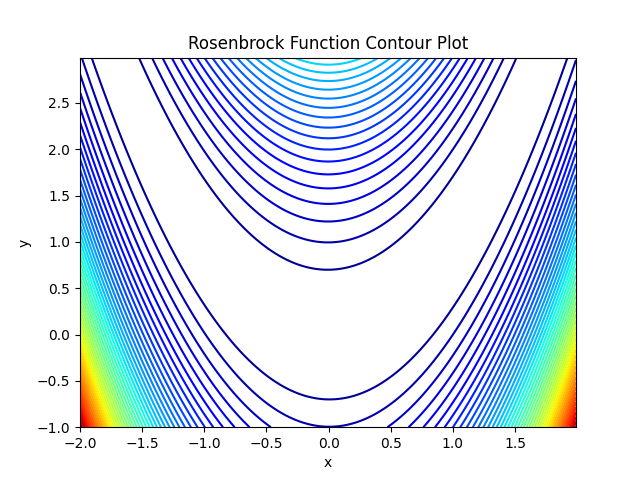
The contour plot reveals the function’s valley and the steep gradients surrounding it. The global minimum appears as the center of the concentric contours.

1.4.3 Initializing Particles on the Rosenbrock Function #

To apply PSO to the Rosenbrock function, we start by initializing a swarm of particles randomly within the search space. Each particle’s position represents a potential solution to the optimization problem.

1.4.3.1 Generating Random Points #

Here’s how we can generate random points within a specified range using NumPy:

import numpy as np

def initialize_particles(num_particles, lower_bound, upper_bound):
    return np.random.uniform(lower_bound, upper_bound, (num_particles, 2))

particles = initialize_particles(10, -5, 5)

In this example, we initialize 10 particles with random positions in the range [-5, 5] for both x and y coordinates.

1.4.3.2 Evaluating the Rosenbrock Function #

Next, we evaluate the Rosenbrock function at each particle’s position to assess the quality of the potential solutions:

def evaluate_rosenbrock(particles):
    return rosenbrock(particles[:, 0], particles[:, 1])

fitness = evaluate_rosenbrock(particles)

The fitness array holds the function values corresponding to each particle’s position. In the context of PSO initialization, these fitness values serve as the initial personal best values for the particles.

By generating random particles and evaluating their fitness on the Rosenbrock function, we set the stage for the PSO algorithm to iteratively improve the solutions and converge towards the global minimum.

In the next section, we’ll dive into the core components of PSO and see how the particles navigate the search space to find the optimal solution.

Exercises #

This exercise aims to solidify your understanding of the core components of Particle Swarm Optimization (PSO) by implementing and visualizing the initialization of random particles in a 2D search space. You will create a Python script to generate particles with random positions and plot their initial distribution using the matplotlib library.

Exercise 1: Creating Particles #

Implement a Python function, create_particles(num_particles, search_space), that initializes a set of particles with random positions in a given 2D search space. The function should take the following parameters:

• num_particles: The number of particles to create.
• search_space: A tuple specifying the boundaries of the search space, e.g., ((x_min, x_max), (y_min, y_max)).

The function should return a list of particles, where each particle is represented as a tuple of its x and y coordinates.

Exercise 2: Visualization of Particles #

Use the matplotlib library to visualize the initial positions of the particles in a 2D plot. Follow these steps:

1. Import the necessary matplotlib functions, such as pyplot.

2. Create a new figure and axis using plt.subplots().

3. Extract the x and y coordinates of the particles into separate lists using list comprehension or a for loop.

4. Use ax.scatter(x_coords, y_coords) to plot the particles as points on the 2D axis.

5. Set appropriate labels for the x-axis, y-axis, and the plot title using ax.set_xlabel(), ax.set_ylabel(), and ax.set_title(), respectively.

6. Display the plot using plt.show().

Exercise 3: Analysis of Initial Setup #

1. Run your script with different values for num_particles and observe how the initial distribution of particles changes. What do you notice about the spread and density of particles as the number of particles increases?

2. Experiment with different search space boundaries and analyze how the initial random distribution of particles adapts to the given search space. Consider scenarios where the search space is symmetric (e.g., ((-5, 5), (-5, 5))) and asymmetric (e.g., ((0, 10), (-2, 8))).

3. Discuss the importance of the initial random distribution of particles in the context of PSO. How does it contribute to the exploration of the search space in the early stages of the optimization process?

By completing this exercise, you will gain hands-on experience in initializing particles and visualizing their initial distribution using Python and matplotlib. This lays the foundation for understanding the dynamic behavior of particles as they explore and converge towards optimal solutions in subsequent chapters.

Answers #

import numpy as np

def create_particles(num_particles, search_space):
    # Unpack the search space boundaries
    (x_min, x_max), (y_min, y_max) = search_space

    # Generate random positions within the given boundaries
    x_positions = np.random.uniform(x_min, x_max, num_particles)
    y_positions = np.random.uniform(y_min, y_max, num_particles)

    # Combine x and y coordinates into a list of tuples
    particles = list(zip(x_positions, y_positions))

    return particles

import matplotlib.pyplot as plt

def plot_particles(particles):
    # Create a new figure and axis
    fig, ax = plt.subplots()

    # Extract x and y coordinates from particles
    x_coords, y_coords = zip(*particles)

    # Plot particles as scatter points
    ax.scatter(x_coords, y_coords, color='blue', marker='o', label='Particles')

    # Set labels and title
    ax.set_xlabel('X coordinate')
    ax.set_ylabel('Y coordinate')
    ax.set_title('Initial Distribution of Particles')
    ax.legend()

    # Display the plot
    plt.show()

Summary #

Chapter 1 introduced Particle Swarm Optimization (PSO), a nature-inspired optimization algorithm that harnesses the collective intelligence of swarms. The chapter explored the origins of PSO, drawing inspiration from the flocking behavior of birds and schooling of fish. Core components of PSO, such as particles, population, position, velocity, and the objective function, were explained in detail. The basic mathematical model governing particle movement was presented, along with the position and velocity update equations. The chapter also discussed the parameters influencing particle movement, like inertia weight and acceleration coefficients. Finally, an exercise was provided to create and visualize random particles in a 2D search space using Python.

Key Takeaways #

1. PSO is inspired by the collective behavior of swarms in nature, leveraging simple local interactions to achieve global optimization.
2. Particles in PSO navigate the search space, adjusting their positions and velocities based on personal and social influences to collaboratively find optimal solutions.
3. The mathematical model of PSO, governed by the position and velocity update equations, balances exploration and exploitation through parameters like inertia weight and acceleration coefficients.

Exercise Encouragement #

Dive into the world of PSO by implementing particle initialization and visualization in Python. This hands-on exercise will solidify your understanding of the core components and lay the foundation for exploring the dynamic behavior of particles. Don’t be intimidated by the math - take it step by step, and you’ll gain valuable insights into the inner workings of PSO. Your efforts here will pave the way for mastering the fascinating concepts and applications of this powerful optimization technique!

Glossary: #

• Particle Swarm Optimization (PSO): A nature-inspired optimization algorithm based on the collective intelligence of swarms.
• Particle: A potential solution in the search space of PSO.
• Population: A collection of particles in PSO.
• Position: The current location of a particle in the search space, representing a potential solution.
• Velocity: The speed and direction of a particle’s movement in the search space.
• Objective Function: A function that evaluates the quality or fitness of a particle’s position.
• Personal Best: The best position encountered by an individual particle so far.
• Global Best: The best position found by the entire swarm.
• Inertia Weight: A parameter that controls the influence of a particle’s previous velocity on its movement.
• Acceleration Coefficients: Parameters that balance the influence of personal and social experiences on particle movement.

Next Chapter: #

In Chapter 2, we’ll explore the concept of personal best and its role in guiding particle movement, diving deeper into the velocity update mechanism and the influence of individual experiences on the optimization process.