Chapter 7: Continuous Function Optimization #

Introduction to Continuous Function Optimization with GAs #

In the world of optimization, problems can be broadly classified into two categories: discrete and continuous. Discrete optimization deals with problems where the variables can only take on specific, distinct values, such as integers. On the other hand, continuous optimization involves problems where the variables can assume any value within a given range, often represented by real numbers. Genetic Algorithms (GAs) have proven to be versatile tools capable of tackling both discrete and continuous optimization problems, making them valuable assets in a wide array of domains.

Importance of Continuous Function Optimization #

Continuous function optimization plays a crucial role in numerous fields, enabling practitioners to find the best solutions to complex problems. Let’s explore some of the key areas where continuous optimization makes a significant impact.

Engineering Applications #

In engineering, continuous function optimization is extensively used in design processes. For instance, aerodynamic shape optimization involves fine-tuning the shape of an aircraft wing to minimize drag and maximize lift. Similarly, structural optimization helps engineers determine the optimal dimensions and materials for buildings, bridges, and other structures to ensure maximum strength and stability while minimizing cost.

Machine Learning and Data Science #

Continuous function optimization is at the heart of many machine learning algorithms. Hyperparameter tuning, a process that involves finding the best combination of model parameters, relies on continuous optimization techniques. By optimizing these parameters, data scientists can improve the performance and accuracy of their models, leading to better predictions and insights.

Economics and Finance #

In the realm of economics and finance, continuous function optimization is employed in various scenarios. Portfolio optimization, for example, involves determining the optimal allocation of assets to maximize returns while minimizing risk. Market equilibrium analysis, another application, uses continuous optimization to understand how supply and demand interact to determine prices in a market.

By leveraging the power of GAs for continuous function optimization, practitioners across these diverse fields can uncover innovative solutions, improve efficiency, and drive breakthroughs in their respective domains.

Understanding Rastrigin’s Function #

Defining Rastrigin’s Function #

Rastrigin’s function is a classic optimization problem that serves as a benchmark for testing the performance of optimization algorithms, including genetic algorithms. This function, named after Russian mathematician Leonid Rastrigin, is known for its complex landscape featuring numerous local minima and a single global minimum.

Here’s a pure Python function to evaluate Rastrigin’s function in one dimension:

import math

# Evaluate the one-dimensional Rastrigin function.
def rastrigin_1d(x, A=10):
    return A + (x ** 2) - A * math.cos(2 * math.pi * x)

# Example usage:
x_value = 0.5
result = rastrigin_1d(x_value)
print("Rastrigin's function value at x =", x_value, "is", result)

This function takes a single input x, and evaluates Rastrigin’s function at that point, returning the result. The constant A is set with a default of 10 but can be adjusted if needed.

To evaluate Rastrigin’s function for a list of numerical values, where each value in the list represents a different dimension, we can generalize the function.

For a list of values values, where n is the number of dimensions represented by the length of the list, the function can be defined in Python as follows:

import math

# Evaluate the Rastrigin function for a list of numerical values.
def rastrigin(values, A=10):
    n = len(values)
    return A * n + sum(x**2 - A * math.cos(2 * math.pi * x) for x in values)

# Example usage:
values = [0.5, -1.5, 2.0]
result = rastrigin(values)
print("Rastrigin's function value at", values, "is", result)

This function, rastrigin, takes a list of numerical values and computes the value of Rastrigin’s function across all dimensions specified in the list. The use of list comprehension makes it easy to apply the function’s formula to each element in the list and sum the results.

Visualizing Rastrigin’s Function #

Visualizing Rastrigin’s Function in 1D #

To visualize Rastrigin’s Function, particularly in one dimension, we can use Matplotlib, a popular Python library for data visualization. We’ll generate a plot of Rastrigin’s function over a range of values to see its characteristic wavy, non-convex shape with many local minima. Here’s a Python code snippet that demonstrates this:

import numpy as np
import matplotlib.pyplot as plt
import math

def rastrigin_1d(x, A=10):
    """
    Evaluate the one-dimensional Rastrigin function.

    Parameters:
    - x (float): The point at which to evaluate the function.
    - A (float, optional): The constant value A in the function. Default is 10.

    Returns:
    - float: The value of the Rastrigin function at point x.
    """
    return A + (x ** 2) - A * math.cos(2 * math.pi * x)

# Generate a range of x values from -5.5 to 5.5
x_values = np.linspace(-5.5, 5.5, 400)

# Compute the Rastrigin function values for each x
y_values = np.array([rastrigin_1d(x) for x in x_values])

# Create the plot
plt.figure(figsize=(10, 5))
plt.plot(x_values, y_values, label='Rastrigin Function')
plt.title('Rastrigin Function Visualization')
plt.xlabel('x')
plt.ylabel('f(x)')
plt.grid(True)
plt.legend()
plt.show()

The output looks as follows:

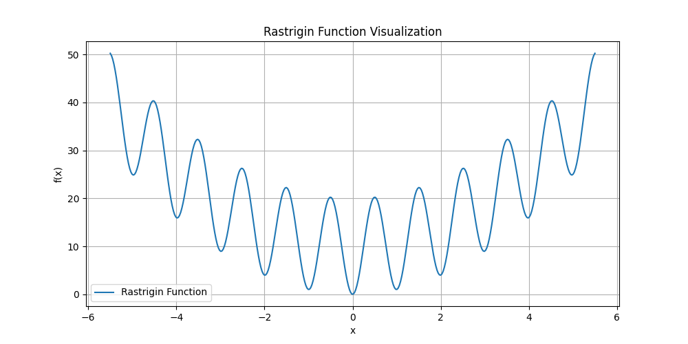
This script does the following:

1. Function Definition: Defines rastrigin_1d, which computes Rastrigin’s function for a single value of x.
2. Data Generation: Generates a range of x values between -5.5 and 5.5, which is typically sufficient to observe the multiple minima and maxima of the function.
3. Function Evaluation: Applies the rastrigin_1d function to each x value in the range using a list comprehension.
4. Visualization: Uses Matplotlib to plot the results. The plot settings ensure that the grid, labels, and legend are properly configured for better understanding and visualization.

You can run this script in any Python environment that has NumPy and Matplotlib installed. It will display the plot directly if you are using a Jupyter notebook or similar interactive environment. If you’re running it in a script file, the plot will appear in a separate window when you execute the script.

Visualizing Rastrigin’s Function in 2D #

To visualize the Rastrigin function as a surface plot for two dimensions, we can use Matplotlib’s mpl_toolkits.mplot3d module. This will help in demonstrating the complex topography of the function, highlighting its peaks and valleys more effectively in a 3D space. Here is a Python code snippet to create a 3D surface plot of the Rastrigin function:

import numpy as np
import matplotlib.pyplot as plt
from mpl_toolkits.mplot3d import Axes3D
import math

def rastrigin_2d(x, y, A=10):
    """
    Evaluate the two-dimensional Rastrigin function.

    Parameters:
    - x, y (float): The points at which to evaluate the function.
    - A (float, optional): The constant value A in the function. Default is 10.

    Returns:
    - float: The value of the Rastrigin function at point (x, y).
    """
    return A*2 + (x ** 2 - A * np.cos(2 * np.pi * x)) + (y ** 2 - A * np.cos(2 * np.pi * y))

# Generate a mesh grid of x and y values
x = np.linspace(-5.5, 5.5, 400)
y = np.linspace(-5.5, 5.5, 400)
X, Y = np.meshgrid(x, y)

# Compute the Rastrigin function values for each (x, y) pair
Z = rastrigin_2d(X, Y)

# Create a 3D plot
fig = plt.figure(figsize=(14, 9))
ax = fig.add_subplot(111, projection='3d')
surf = ax.plot_surface(X, Y, Z, cmap='viridis', edgecolor='none')
ax.set_title('3D Surface Plot of Rastrigin Function')
ax.set_xlabel('X')
ax.set_ylabel('Y')
ax.set_zlabel('f(X, Y)')
fig.colorbar(surf, ax=ax, shrink=0.5, aspect=10)  # Add a color bar which maps values to colors.

plt.show()

The output looks as follows:

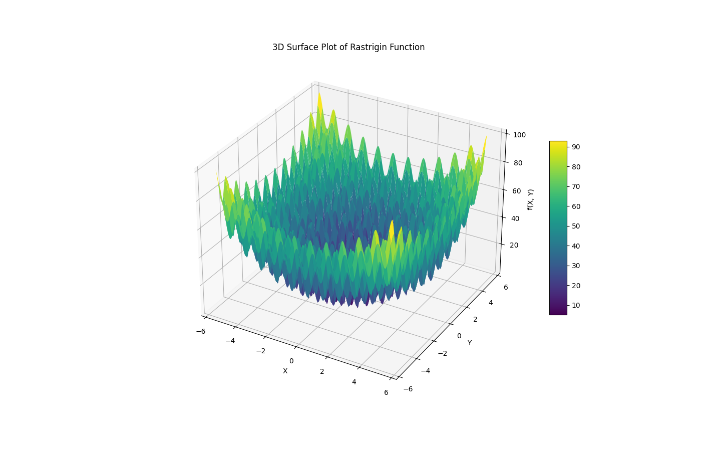
This script does the following:

1. Function Definition: The function rastrigin_2d is defined to compute the Rastrigin function for two variables ( x ) and ( y ).
2. Grid Generation: Using numpy.linspace and numpy.meshgrid, a grid of ( x ) and ( y ) values is created. This grid covers the domain from -5.5 to 5.5 for both variables, which is suitable for observing the function’s characteristics.
3. Function Evaluation: The Rastrigin function is evaluated at each point on the grid. The computation leverages vectorized operations for efficiency.
4. 3D Plotting: The plot is set up with a 3D projection, and plot_surface is used to create the surface plot. The colormap ‘viridis’ is applied for visual appeal, and edges are smoothed for clarity.
5. Display: Labels and titles are added for clarity, and a color bar is included to interpret the function values visually.

This code will generate a detailed 3D surface plot of the Rastrigin function, clearly depicting its complex topology.

Challenges of Optimization #

One of the main challenges in optimizing Rastrigin’s function lies in its numerous local minima. The function has a large number of local minima that are close to the global minimum in terms of function value but far from it in terms of distance in the search space. This characteristic makes it difficult for optimization algorithms to navigate the landscape and find the global minimum without getting stuck in local minima.

Rastrigin’s function is also considered a deceptive function. Deceptive functions are those where the average fitness of a region in the search space does not necessarily indicate the location of the global optimum. In other words, the function “deceives” the optimization algorithm by leading it away from the global minimum. This deceptive nature, combined with the high number of local minima, makes Rastrigin’s function a challenging test case for optimization algorithms, including genetic algorithms.

Decoding Mechanisms in GAs #

Genetic algorithms often require a means to bridge the gap between the discrete world of bitstrings and the continuous domain of real numbers. This is where decoding mechanisms come into play. By transforming bitstrings into continuous values, GAs can effectively explore and optimize functions defined on continuous spaces. In this section, we’ll look into binary decoding, its limitations, and an alternative encoding scheme called Gray code.

Introduction to Binary Decoding #

Binary decoding is a fundamental technique used in GAs to convert bitstrings into continuous values. The process involves interpreting the binary representation of a bitstring as a decimal number and then mapping it to a specific range of continuous values. This mapping allows the GA to search for solutions in the continuous domain while still leveraging the binary nature of genetic operators like mutation and crossover.

Example Python Function for Binary Decoding #

To illustrate binary decoding, let’s consider a simple Python function that takes a bitstring and decodes it to a float value within a specified range:

def binary_decode(bitstring, min_val, max_val, num_bits):
    decimal = int(bitstring, 2)
    return min_val + decimal * (max_val - min_val) / (2**num_bits - 1)

The function takes the bitstring, the minimum and maximum values of the desired range (min_val and max_val), and the number of bits in the bitstring (num_bits). It first converts the bitstring to its decimal equivalent using int(bitstring, 2) and then maps the decimal value to the specified range using the formula shown.

Worked Example of Encoding and Decoding #

To demonstrate the encoding and decoding process, let’s consider a continuous value of 0.75 in the range [0, 1]. To encode this value using 8 bits, we first convert it to a decimal integer:

decimal = round(0.75 * (2**8 - 1)) # 191

The decimal value 191 is then converted to its binary representation:

bitstring = bin(191)[2:].zfill(8) # "10111111"

To decode the bitstring back to the continuous value, we apply the binary decoding function:

decoded_value = binary_decode("10111111", 0, 1, 8) # 0.75

The result is 0.7490196078431373, not exactly the original value 0.75.

In this case, we have lost some precision with our chosen representation in 8 bits. This is an important concern when choosing the precision required for the floating point values.

Limitations of Binary Encoding/Decoding #

While binary encoding is widely used in GAs, it has some limitations when applied to function optimization problems. One significant drawback is the presence of Hamming cliffs, where two adjacent continuous values may have binary representations that differ in multiple bits. This can hinder the GA’s ability to make small, gradual changes to solutions during the search process.

Another limitation is the non-uniform distribution of decoded values across the search space. The binary encoding scheme tends to allocate more representational precision to certain regions of the search space, potentially biasing the GA’s exploration.

Introduction to Gray Code #

Gray code, named after Frank Gray, is an alternative encoding scheme that addresses some of the limitations of binary encoding. In Gray code, adjacent values differ by only one bit, eliminating the Hamming cliff problem. This property allows the GA to make smoother transitions between solutions, potentially improving its exploration and convergence capabilities.

Gray Code Encoding and Decoding #

To encode a bitstring using Gray code, we can use the following Python function:

def gray_encode(bitstring):
    gray = bitstring[0]
    for i in range(1, len(bitstring)):
        gray += str(int(bitstring[i]) ^ int(bitstring[i-1]))
    return gray

The encoding process involves XORing each bit with the previous bit, starting from the most significant bit. Decoding a Gray-encoded bitstring back to binary can be achieved by reversing this process:

def gray_decode(gray):
    binary = gray[0]
    for i in range(1, len(gray)):
        binary += str(int(binary[i-1]) ^ int(gray[i]))
    return binary

Encoding and GA Performance #

The choice of encoding scheme can significantly impact the performance of a GA in function optimization problems. Gray code, with its ability to mitigate Hamming cliffs and provide a more uniform distribution of values, often leads to improved convergence and exploration compared to binary encoding.

However, the effectiveness of Gray code may vary depending on the specific problem and the characteristics of the fitness landscape. In some cases, binary encoding may still be preferred due to its simplicity and compatibility with standard genetic operators.

As a rule of thumb, it’s recommended to experiment with both encoding schemes and assess their performance on the specific problem at hand. By understanding the strengths and limitations of each approach, you can make informed decisions and tailor the GA to the requirements of the optimization task.

Exercises #

In this exercise, you’ll implement binary and Gray code encoding and decoding functions for floating-point values, and then use them in a genetic algorithm to optimize Rastrigin’s function. By comparing the performance of each encoding/decoding scheme, you’ll gain insights into their impact on the GA’s effectiveness in solving continuous optimization problems.

Exercise 1: Implementing Binary and Gray Code Encoding/Decoding #

1. Binary Encoding and Decoding: Implement the functions binary_encode(value, min_val, max_val, num_bits) and binary_decode(bitstring, min_val, max_val, num_bits) that encode a floating-point value to a binary bitstring and decode a binary bitstring back to a floating-point value, respectively. The min_val and max_val parameters specify the range of values, and num_bits determines the precision of the encoding.

2. Gray Code Encoding and Decoding: Implement the functions gray_encode(bitstring) and gray_decode(gray) that convert a binary bitstring to its Gray code equivalent and vice versa.

3. Testing the Functions: Test your encoding and decoding functions by encoding a set of floating-point values, decoding the resultant bitstrings, and verifying that the decoded values match the original values. Perform this test for both binary and Gray code encoding.

Exercise 2: Implementing the Genetic Algorithm for Rastrigin’s Function #

1. Fitness Function: Implement the fitness function rastrigin(x) that takes a list of floating-point values x and returns the value of Rastrigin’s function for those inputs.

2. GA Components: Implement the necessary components of the genetic algorithm, including population initialization, selection, crossover, and mutation operators. Use your binary and Gray code encoding/decoding functions to convert between floating-point values and bitstrings.

3. Running the GA: Run the genetic algorithm to optimize Rastrigin’s function in a fixed number of dimensions (e.g., 1, 2, 3) using either or both a binary and Gray code encoding. Set appropriate values for population size, mutation rate, crossover rate, and termination criteria.

Exercise 3: Comparing Performance and Analyzing Results #

1. Performance Metrics: For each run of the GA, record relevant performance metrics such as the best fitness value found, the number of generations to convergence, and the computation time.

2. Multiple Runs: Run the GA multiple times (e.g., 10 or more) for each encoding scheme and dimension to account for the stochastic nature of the algorithm.

3. Statistical Analysis: Perform a statistical analysis of the results to compare the performance of binary and Gray code encoding. Use appropriate measures such as mean, median, and standard deviation of the performance metrics.

4. Visualization: Create plots to visualize the convergence of the GA over generations for each encoding scheme. Also, plot the best solutions found by the GA against the known global minimum of Rastrigin’s function.

5. Discussion: Based on your results, discuss the advantages and disadvantages of binary and Gray code encoding for optimizing Rastrigin’s function. Consider factors such as convergence speed, solution quality, and robustness to local optima.

By completing this exercise, you’ll gain practical experience in implementing binary and Gray code encoding/decoding, applying a GA to optimize a continuous function, and analyzing the performance of different encoding schemes. This knowledge will equip you to tackle more complex continuous optimization problems using genetic algorithms.

Answers #

import numpy as np

def binary_encode(value, min_val, max_val, num_bits):
   # Scale value to the range [0, 2**num_bits - 1]
   scale = (value - min_val) / (max_val - min_val)
   integer = int(scale * ((2 ** num_bits) - 1))
   # Convert integer to binary string
   return format(integer, f'0{num_bits}b')

def binary_decode(bitstring, min_val, max_val, num_bits):
   # Convert binary string to integer
   integer = int(bitstring, 2)
   # Scale integer back to the floating-point value
   value = integer / ((2 ** num_bits) - 1)
   return min_val + value * (max_val - min_val)

def gray_encode(bitstring):
   binary = int(bitstring, 2)
   gray = binary ^ (binary >> 1)
   return format(gray, f'0{len(bitstring)}b')

def gray_decode(gray):
   binary = int(gray, 2)
   mask = binary
   while mask != 0:
       mask >>= 1
       binary ^= mask
   return format(binary, f'0{len(gray)}b')

import numpy as np

def binary_encode(value, min_val, max_val, num_bits):
   # Scale value to the range [0, 2**num_bits - 1]
   scale = (value - min_val) / (max_val - min_val)
   integer = int(scale * ((2 ** num_bits) - 1))
   # Convert integer to binary string
   return format(integer, f'0{num_bits}b')

def binary_decode(bitstring, min_val, max_val, num_bits):
   # Convert binary string to integer
   integer = int(bitstring, 2)
   # Scale integer back to the floating-point value
   value = integer / ((2 ** num_bits) - 1)
   return min_val + value * (max_val - min_val)

def gray_encode(bitstring):
   binary = int(bitstring, 2)
   gray = binary ^ (binary >> 1)
   return format(gray, f'0{len(bitstring)}b')

def gray_decode(gray):
   binary = int(gray, 2)
   mask = binary
   while mask != 0:
       mask >>= 1
       binary ^= mask
   return format(binary, f'0{len(gray)}b')

# Test values
values = [0.1, 0.5, 0.9]
min_val = 0.0
max_val = 1.0
num_bits = 16

for value in values:
   binary = binary_encode(value, min_val, max_val, num_bits)
   gray = gray_encode(binary)
   decoded_binary = binary_decode(binary, min_val, max_val, num_bits)
   decoded_gray = binary_decode(gray_decode(gray), min_val, max_val, num_bits)
   print(f"Value: {value}\n\tBinary: {binary}, Decoded: {decoded_binary}\n\tGray: {gray}, Gray Decoded: {decoded_gray}")

def rastrigin(x):
   A = 10
   return A * len(x) + sum([(xi**2 - A * np.cos(2 * np.pi * xi)) for xi in x])

def binary_decode(bitstring, min_val, max_val, num_bits):
   # Convert binary string to integer
   integer = int(bitstring, 2)
   # Scale integer back to the floating-point value
   value = integer / ((2 ** num_bits) - 1)
   return min_val + value * (max_val - min_val)

def evaluate_fitness(bitstring):
    # convert to string
    bs = ''.join(bitstring)
    # decode
    x = binary_decode(bs, -5.5, 5.5, len(bs))
    # evaluate
    return rastrigin(x)

def tournament_selection(population, tournament_size):
    tournament = random.sample(population, tournament_size)
    fittest = min(tournament, key=evaluate_fitness)
    return fittest

def replace_population(old_pop, new_pop, elitism_count=1):
    sorted_old_pop = sorted(old_pop, key=evaluate_fitness)
    new_pop[elitism_count:] = sorted_old_pop[:elitism_count]
    return new_pop

def genetic_algorithm(pop_size, bitstring_length, generations):
    population = initialize_population(pop_size, bitstring_length)
    best_fitness = float('inf')
    for generation in range(generations):
        new_population = []
        while len(new_population) < pop_size:
            parent1 = tournament_selection(population, 3)
            parent2 = tournament_selection(population, 3)
            offspring1, offspring2 = one_point_crossover(parent1, parent2)
            offspring1 = bitflip_mutation(offspring1, 0.01)
            offspring2 = bitflip_mutation(offspring2, 0.01)
            new_population.extend([offspring1, offspring2])
        population = replace_population(population, new_population, 2)
        best_fitness = min(best_fitness, min(evaluate_fitness(ind) for ind in population))
        print(f"Generation {generation}: Best Fitness {best_fitness}")

import random
import math

def initialize_population(pop_size, bitstring_length):
    return [['1' if random.random() > 0.5 else '0' for _ in range(bitstring_length)] for _ in range(pop_size)]

def rastrigin(x):
   A = 10
   return A + (x ** 2) - A * math.cos(2 * math.pi * x)

def binary_decode(bitstring, min_val, max_val, num_bits):
   # Convert binary string to integer
   integer = int(bitstring, 2)
   # Scale integer back to the floating-point value
   value = integer / ((2 ** num_bits) - 1)
   return min_val + value * (max_val - min_val)

def evaluate_fitness(bitstring):
    # convert to string
    bs = ''.join(bitstring)
    # decode
    x = binary_decode(bs, -5.5, 5.5, len(bs))
    # evaluate
    return rastrigin(x)

def tournament_selection(population, tournament_size):
    tournament = random.sample(population, tournament_size)
    fittest = min(tournament, key=evaluate_fitness)
    return fittest

def one_point_crossover(parent1, parent2):
    point = random.randint(1, len(parent1) - 1)
    offspring1 = parent1[:point] + parent2[point:]
    offspring2 = parent2[:point] + parent1[point:]
    return offspring1, offspring2

def bitflip_mutation(bitstring, prob):
    return ['1' if (bit == '0' and random.random() < prob) else '0' if (bit == '1' and random.random() < prob) else bit for bit in bitstring]

def replace_population(old_pop, new_pop, elitism_count=1):
    sorted_old_pop = sorted(old_pop, key=evaluate_fitness)
    new_pop[elitism_count:] = sorted_old_pop[:elitism_count]
    return new_pop

def genetic_algorithm(pop_size, bitstring_length, generations):
    population = initialize_population(pop_size, bitstring_length)
    best_fitness = float('inf')
    for generation in range(generations):
        new_population = []
        while len(new_population) < pop_size:
            parent1 = tournament_selection(population, 3)
            parent2 = tournament_selection(population, 3)
            offspring1, offspring2 = one_point_crossover(parent1, parent2)
            offspring1 = bitflip_mutation(offspring1, 0.01)
            offspring2 = bitflip_mutation(offspring2, 0.01)
            new_population.extend([offspring1, offspring2])
        population = replace_population(population, new_population, 2)
        best_fitness = min(best_fitness, min(evaluate_fitness(ind) for ind in population))
        print(f"Generation {generation}: Best Fitness {best_fitness}")

# Run the genetic algorithm
pop_size = 100
bitstring_length = 32
generations = 500
genetic_algorithm(pop_size, bitstring_length, generations)

Summary #

Chapter 7 introduced the concept of continuous function optimization using genetic algorithms (GAs). It explored the importance of continuous optimization in various fields, such as engineering, machine learning, and economics. The chapter presented Rastrigin’s function as a challenging benchmark problem, explaining its complex landscape and the difficulties it poses for optimization algorithms. The concept of deception in optimization was also discussed. The chapter then explored decoding mechanisms, focusing on binary decoding and its limitations. Gray code was introduced as an alternative encoding scheme that addresses some of the drawbacks of binary encoding. The impact of encoding choices on GA performance was highlighted, emphasizing the need for experimentation and problem-specific considerations.

Key Takeaways #

1. Continuous function optimization is crucial in many real-world applications, and GAs can be effective tools for solving these problems.
2. Rastrigin’s function serves as a challenging benchmark for evaluating the performance of optimization algorithms due to its numerous local minima and deceptive nature.
3. The choice of encoding scheme, such as binary or Gray code, can significantly influence the performance of a GA in continuous optimization tasks.

Exercise Encouragement #

Take on the challenge of implementing binary and Gray code encoding/decoding functions and applying them to optimize Rastrigin’s function using a GA. This hands-on experience will deepen your understanding of the intricacies involved in continuous optimization and the impact of encoding schemes. Don’t be discouraged if the results vary; embrace the opportunity to experiment, analyze, and learn from the outcomes. Your efforts will equip you with valuable insights into tailoring GAs for real-world optimization problems.

Glossary: #

• Continuous Optimization: Optimization problems where variables can take on any value within a given range.
• Rastrigin’s Function: A benchmark optimization problem known for its complex landscape and numerous local minima.
• Deceptive Function: A function where the average fitness of a region does not necessarily indicate the location of the global optimum.
• Binary Decoding: The process of converting a binary bitstring to a continuous value.
• Hamming Cliff: A phenomenon where adjacent continuous values have binary representations that differ in multiple bits.
• Gray Code: An encoding scheme where adjacent values differ by only one bit.
• Encoding: The process of representing a solution in a format suitable for a GA.
• Decoding: The process of converting an encoded solution back to its original form.

End #

This was the last chapter of the book. Well done, you made it!

Review how far you have come.